Neural Net Module

 

Items Covered in This Section

• - Neural Net Basics
• - Using Neural Net Module
• - NN Outputs
• - NN Inputs
• - Training NN
• - When to stop NN training
• - Auto Stop

Introduction

You have already learned how to do the very basics of Timing Solution Software: You have learned how to download price history data that you can use for your future forecast; you have learned how to apply periodograms to the price charts; and you have learned how to create a forecast based on Astronomical cycles.

Now you will learn about another popular module - Neural Net Module. While Neural Nets have been gaining popularity for their ability for image processing and facial recognition, they also have proven themselves being useful in analyzing financial markets and forecasting future price movements.

What is a Neural Net? Before you use the module, it is a good idea to discuss the basics of Neural Network theory. If you are already familiar with the concept, you can go to the next section and learn how to use the Neural Net Module in Timing Solution.

Neural Net Explained

Neural Net is a mathematical procedure of modelling existing processes. Processing complex data and deriving specific patterns from that, the Neural Net creates a model that is able to mimic the original process and thus to make conclusions about its future outcome. An example of this process is weather forecast. We can collect data about the air (such as humidity, temperature, density, etc.) and we can also assume that the weather today strongly depends on the weather conditions yesterday and the days before yesterday. It means that we expect the existence of the same patterns between today's data and the previous information. The process of finding these patterns is what Neural Net is designed to do: it takes a number of factors into account and observes how these factors might affect the result.

This concept is also illustrated in the picture below:

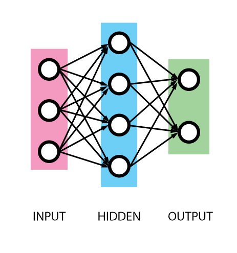
Every Neural Net has this structure: the input layer, the hidden layer and the output layer. The Input Layer (or inputs) is where the variables to be processed are stored. This is where we enter any factors that we think might affect the result. The Output Layer (outputs) is where we store all our results. And finally the Hidden Layer is the layer/layers where the machine does computations to find any correlation between inputs and outputs. The Neural Net (NN) shown above is called multilayer perceptron.

Going back to the weather example: we would store all historical data about the weather conditions. Recorded temperature, humidity, atmospheric pressure, wind, etc. - these may serve as inputs. Outputs are what we would like to know - the weather tomorrow (tomorrow's temperature, humidity, pressure, wind). Once we start up the training process of the Neural Net, the hidden layer will start looking for any patterns between the input layer and the events defined in the output layer.

It is very important to use as inputs only those factors that are relevant to the process we are modelling. Remember the GIGO rule: Garbage In - Garbage Out.

Hidden layers are a core of the Neural Network technology; they allow to build NON LINEAR models. (If it would be a linear relationship between inputs and outputs, we would not need a Neural Net.)

What is the difference between linear and non linear models?

LINEAR models are those where we can find a weight that reflects how some input event affects the output. For example, we could calculate tomorrow's temperature using a linear formula like the one below:

Tomorrow's temperature = 0.9 * today's temperature - 0.17* yesterday's temperature + 0.012 * today's pressure, etc.

However, in reality we deal with more complicated relations. Instead of the formula above, we may get this set of conditions:

1) if today the temperature and pressure is high - the temperature tomorrow is also high;

2) if today the temperature is high and pressure is low - the temperature tomorrow is low;

3) otherwise the temperature tomorrow is the same as the temperature today.

Here temperature and pressure work together, we cannot separate temperature and pressure effects. In NONLINEAR model the effect of the pressure depends on the temperature. On the contrary, in a linear model we are able to isolate temperature and pressure effects, as in the example above (there the effect of temperature is 0.9 and effects of pressure is 0.012).

The hidden layers allow to reveal these nonlinear patterns. The more hidden neurons and hidden layers we have, the more complicated nonlinear pattern the NN can reveal.

Training of the Neural Network is a process of adjustment of the NN using available historical data (the information that we already know). Back to our example, the NN takes as an output the weather condition today (that we know) and considers it in regards to inputs (which are the weather conditions yesterday, two days ago, etc.; we know them too). The NN corrects itself to get better accuracy between the "forecast" (output) and already known weather. Then we take the weather yesterday as a new output while inputs are the weather two, three, etc. days ago - and correct the NN again. Thus we get the best coincidence between the forecasted by this NN and real weather conditions. To train Timing Solution Neural Nets, we apply back propagation algorithm.

As we increase the size of the Hidden Layer, we are able to analyze more and more input parameters and their effect on the outputs. If we find that one Hidden Layer is not enough, we can add multiple hidden layers. Such a Neural Network is called Deep Learning Neural Net and that is exactly what Google and other companies use in their facial recognition algorithms. However, for financial analysis, there is no need for such complex Neural Networks. We have experimented with adding extra hidden layers in the past and found that extra layers did not improve our forecast by much.

Once training is complete, we get new knowledge regarding the relationship between inputs and outputs.  It is the base of Timing Solution forecasting models.

Of course, Neural Nets can be (and are) used for much more than just finding weather patterns. In Timing Solution we use Neural Network technology to compare how a specific model performs against the market movements of a financial instrument. This gives us a freedom to come up with models of our own and then test their performance against historical price data. There are also a number of preset models that can be used for Neural Net analysis; this lesson will focus primarily on these. So, let us begin!

 

Fast Example - following steps by Donald Bradley

In the end of 1940s, Donald Bradley has shown a way how the methods of classical astrology can be applied to analysis of financial markets. He has built an index that indicates the balance between "good" and "bad" aspects. This is so called "Bradley siderograph". Initially, he tried to apply it to some social issues. When his friends saw it, they mentioned that it strongly reminds a stock price chart. That is how it started. We can add to it a modern twist: we can delegate the task of defining "good" and  "bad" aspects to Neural Network.

The general idea of this approach is: any price chart contains "tracks" of astonomical/astrological phenomena. (Tracks here mean that a certain aspect or a set of aspects have some impact on the price chart at certain times). Here is an example: the conjunction aspect between transiting Venus and Saturn has some impact on Bitcoin price chart (Venus - Saturn conjuction's track on Bitcoin):

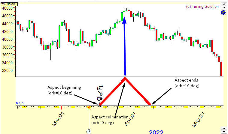
A culmination of this aspect coinsides with a local top of Bitcoin chart. The maximal orb for this aspect is 10 degrees. We can see here that the orb dynamics, from the beginning of this aspect (orb=10 degrees on March 18, 2022)  to its culmination (orb=0 on March 28) to end of this aspect (orb=10, April 8, 2022)  repeats very well the  Bitcoin price movement within three weeks. If this aspect shows the same dynamics for other local Bitcoin tops, it may be used as a tool to forecast the Bitcoin price.

Look at another example, Jupiter - Neptune sexstile. This aspect works in opposite (negative) way: its culmination coinsides with the bottom of Dow Jones Industrial price chart. Plus, due to retrograde motion, this aspect culminates twice in August and December:

 

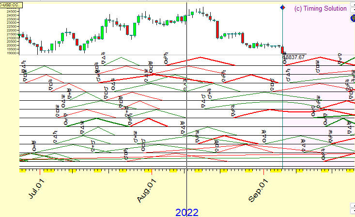
In reality we have much more complicated picture. Below you can see Semenko diagram that shows how aspects of transiting planets work within three months, i.e. you can see how these aspects begin-culminate-end:

 As you see, at any given moment there are many aspects at work. They leave different tracks on the price chart. We need to find a way how deal with them all with the goal of building a forecast. That includes setting the weights, choosing the correct orb. All these parameters are important as they affect the forecast. Neural Network module in Timing Solution allows to do this job.

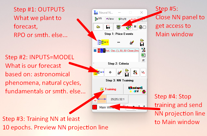
In the following video, we will build together a model based on transiting aspects to create a projection line to forecast the price movement.

There are five necessary steps to build this model:

 

Let's start:

 

 

 

 

Using Neural Net Module

To open Neural Net Module, click here:

Neural Net Outputs

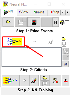
The Neural Net Window is divided into three steps. Unlike most mathematical models, the first step is to select the output. That is the result that Neural Net will compare the model against. To select an output, click the button shown in the picture below:

As an example, let us forecast the detrended oscillator with the period of 50 bars:

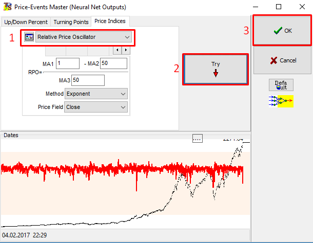
To do so, select "Relative Price Oscillator" from the Drop Down Menu. Below the selection, set various parameters that are relevant. In this example, make sure that MA2 and MA3 are both set to 50.

This is called RPO50 - relative price oscillator with the period of 50 bars (this is the same as percentage price oscillator). It is the same data set, only shown without a trend (we have got rid of any steady movement up or down). Detrending is necessary to do, as Neural Network works better with detrended indicators (it looks for real connections between the price movement of your financial instrument and things that form your model; the existence of a trend confuses this search).

After that, click the Try button. This will preview the detrended data in the lower left part of the window. Click "OK" to load the output into the Neural Net Module.

Neural Net Inputs

The next step is to define inputs (factors that may have some effect on the outputs). They form a model that will be tested against the output. The inputs are used to train the Neural Net and find any correlations between the model and the output defined above.

Click on the main Criteria button to create a model from scratch. Alternatively you may apply models created in ULE module (these should be saved as  *.hyp files), or you can choose from a selection of pre-made models by clicking on the "+" button.

In the example above, Ptolemy aspects are used to forecast RPO50 with the orb of 15 degrees.

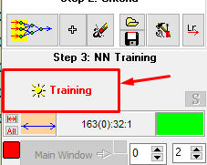
Training Neural Net

As soon as inputs and outputs are defined, it is time for the Neural Net to learn. In the process of learning, the Neural Net will look for any relationship between the inputs and outputs. This is happening on the training interval (which is located before LBC). To start the training, click here:

In seconds the Main screen will look like this:

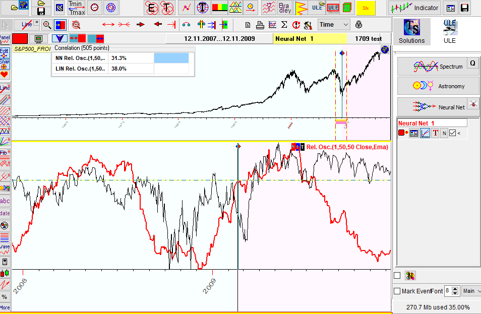
Here the red curve is a product of NN learning/training, while the black line represents RPO50. The red curve is changing trying to find the parameters of the model that make it fit to the price oscillator. It is our goal. The process takes some time. You may want to look at the correlation coefficient, though it is not recommended. We believe that visual evaluation serves better; continue the NN training till you actually see that the red curve reflects the chosen price oscillator very well inside the training interval (the area before LBC).

If you find the fitness of the red curve to the price oscillator satisfactory, you may stop the training process (see details below). The longer the period of NN training, the more is the chance of overtraining it. (If it is too long, the NN starts generating a noise instead of a productive projection line. You will observe an almost perfect fit on the training interval, which is the evidence of a well-designed Neural Net, - and a very poor performance of the projection line in a real life.)

The red curve produced by the Neural Net is extended beyond the LBC. This is how we get a projection line. As soon as you stop the training process, this line does not change. No calculations are done there, you are strictly seeing the projection line created by training in the blue interval (before the LBC) and the relative price oscillator after the LBC. The program does not use the data after the LBC to adjust the projection line. We recommend to keep a small portion of the data after the LBC to evaluate the usefulness of the projection line.

If you want to see how the projection line produced by this model performs at any part of the price history chart, click on the magnify cursor button and then select the appropriate area on the chart to examine it.

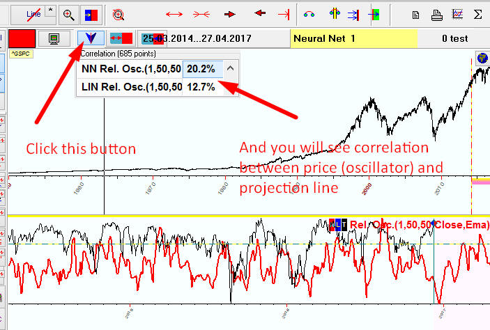
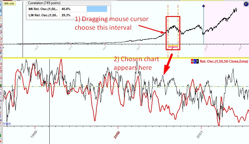
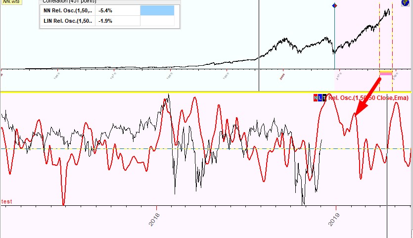
The program shows the correlation calculated for the selected interval. While you choose different intervals, the program recalculates this information panel, so you can see how the projection line fits the price on different intervals. The example below shows the selected price interval 1999-2001 and how our Neural Net works on this interval:

 

 

or you can watch how that same Neural Net works on some other interval after LBC; let it be 2017-2018:

Browsing  Neural Net results on different intervals gives you the idea how it works. The question rises: when to stop Neural Net training?

When to stop Neural Net training

There are no certain rules regarding this object. If you train Neural Net not enough, it will not gather from the price history the information suitable to build a projection line. From the other side, if you train Neural Net too long, you will definitely end up with the overtraining (memorizing) effect (it happens when Neural Net simply memorizes the price history instead of gathering a meaningful information from the price).

We would recommend three rules:

Rule #1: You can stop Neural Net training when the projection line changes not too much during the training process. The projection line may be changing, though the change should not be drastic.

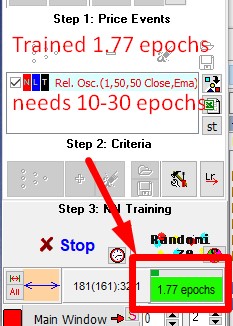
Rule #2: You should train Neural Net  during 10-30 epochs. The amount of trained epochs can be found here:

A training epoch is a very important definition in Neural Network science. Suppose we train Neural Net using 1000 price bars; for EOD chart this is usually about four years of the price history. One training step is when the program corrects the Neural Net's weights taking randomly just one price bar from those 1000 bars. Making 1000 training steps the program hits all of 1000 price bars; this is one epoch. We can say that an epoch is the amount of training steps to hit all available price history.

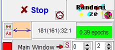
If we have 10K bars on the training interval, the program needs ten times more, i.e. 10K steps to hit all available 10K bars. In other words within one training epoch the Neural Net hits once all of available for training price history points. While you train your Neural Net, the color of the panel changes; lime color means that there are not enough training steps yet:

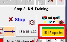
bright orange color means that the Neural Net is "ripe" (trained enough):

Rule #3: To avoid overtraining, do not train Neural Net too long.

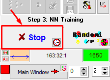
 When you decide that the projection line produced by the Neural Net is OK (it fits the price quite well on different intervals), click "Stop" button to stop the training procedure:

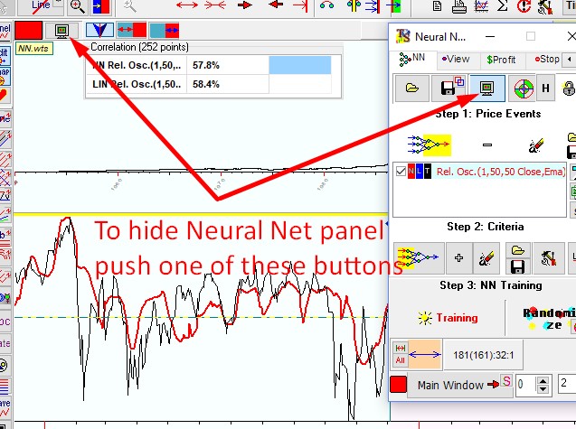
The projection line created by the Neural Net is automatically shown in the Main Window. If you do not want to see it, click one of  these buttons:

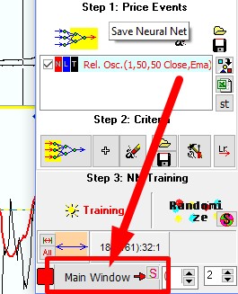
The NN results panel in the lower portion of the Main Window will disappear. If you do not want to see the NN results panel and still want to see the projection line, then click on this "Main Window"  button:

 

Auto stop

If you work quite often with one and the same financial instrument and know it well enough, you may want to use auto stop feature. You can set it here:

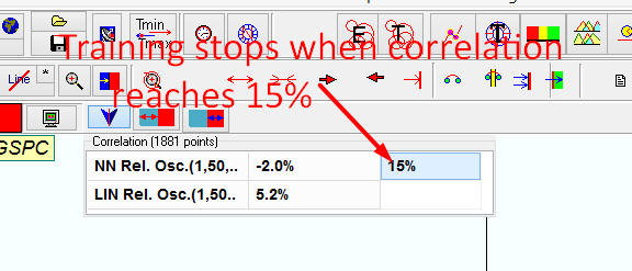
In this example Neural Network stops training when the correlation between  the price and the projection line created by Neural Network reaches 15% at least.

You can define more complicated auto stop criteria:

Here Neural Network stops training when the correlation between Neural Network's projection line and the price reaches 15% at least OR when the correlation between Linear projection line and the price reaches 36% at least.

Another example involves the amount of training epochs:

Here the program stops Neural Network training when the correlation reaches 15% OR  the amount of training epochs reaches 10.

Remember that typing 15% means that we indicate the correlation, while typing 10 means the amount of training epochs.

This concludes the lesson on Neural Net. The next lesson will cover Charting tools and how they can help you in creating your forecast.