TS Terra Incognita Project #1: Trading Strategy Constructor (TSC)
Working in process

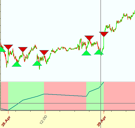
Buy/Sell signals can be generated by many ways using different Technical Analysis techniques. For example, TSC (Trading Strategy Constructor) can generate signals based on a crossover price with moving average, or price band breakout, or RSI breakout. Other software for financial analysis (like Trade Station, Wealth Lab, Trade Studio and many others) provide you the possibility to check any trading strategy and optimize it, too. Timing Solution does it in a totally different way:
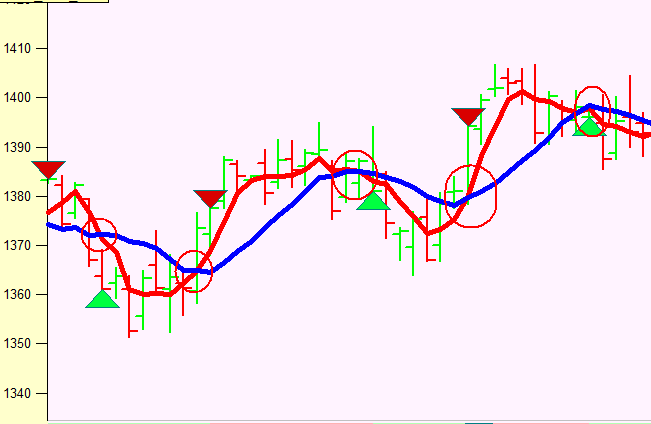
Trading Strategy - it is an order of buy and sell signals. As an example, I will use the simplest trading strategy - a strategy based on moving average crossovers. Under this strategy, a buy signal is generated when a fast moving average crosses a slow moving average FROM DOWN TO UP; and vice versa, a sell signal is generated when the fast moving average crosses the slow moving average UP TO DOWN. Here is an example of these signals calculated for crossovers of 20 (red) and 50 days (blue) moving averages for S&P 50 mini futures daily chart:
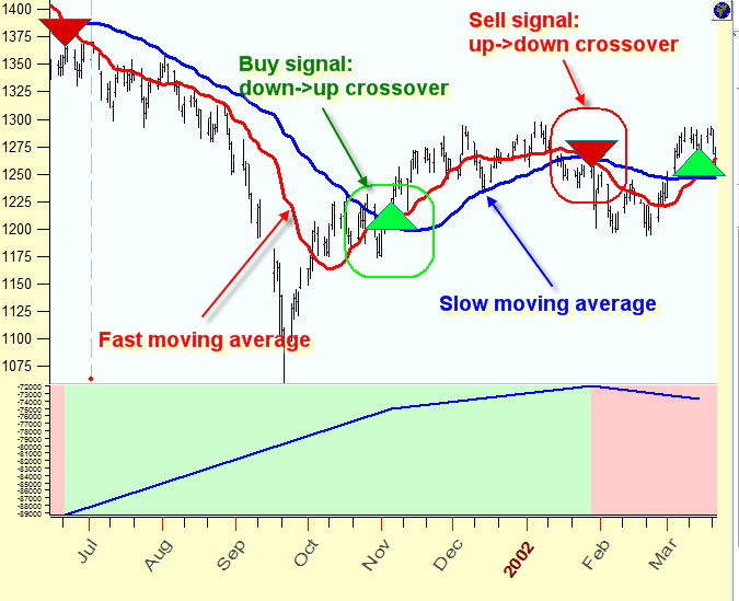
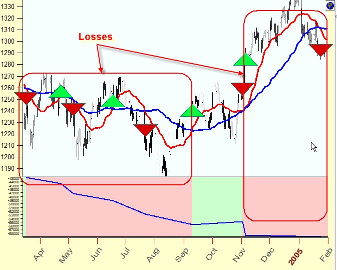
As you can see, this strategy gives good buy/sell signals not all the time:
Timing Solution is able to analyze different strategies, and we plan to add more strategies that model the market behavior in different ways. This is an example of buy/sell signals based on quantum strategy:
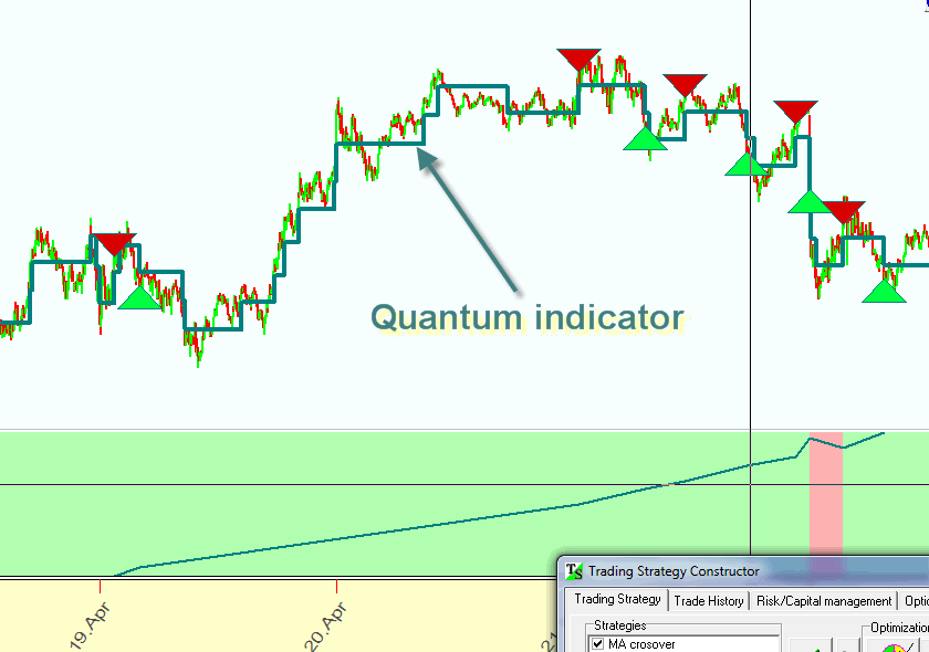
Buy/sell signals here are generated by a specially developed "quantum moving average indicator". This indicator represents the sensitive price levels where the price tends to change the trend. The program finds the best quantum parameters for any financial instrument. We are looking for the best ways to create quantum models (price quantum, time quantum, price-time quantum, volatility quantum etc).
Inverted models - Buy/sell signals on the previous examples were generated using the so-called trend following system. Sometimes we might get better results applying the idea of inverted signals, i.e. using up-down moving average crossovers for buy signals and, accordingly, down-up moving average crossovers for sell signals. The example of this strategy is below:
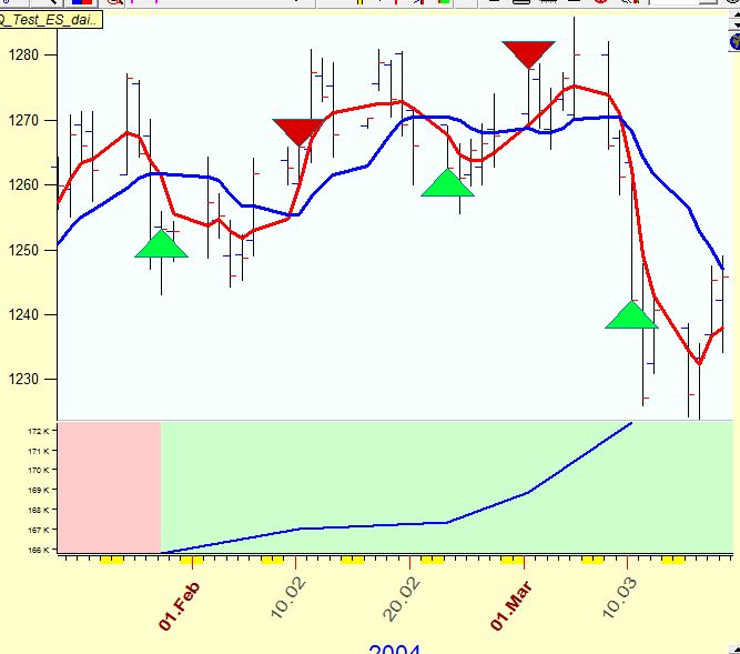
We call these models Inverted models. In Chaos theory, there is a special name for this type of data; it is called anti-persistent (while the data used for trend following systems are closer to persistent data).
Definitions for trading strategies (used in the program)
![]() - trend following
trading strategy based on the crossover of two simple moving averages (SMA): fast MA
period is 5 bars, slow period is 10 bars (fast moving average crosses slow
moving average from down to up);
- trend following
trading strategy based on the crossover of two simple moving averages (SMA): fast MA
period is 5 bars, slow period is 10 bars (fast moving average crosses slow
moving average from down to up);
![]() - Inverted model
based on the crossover of two simple MA 11 and 15 bars; (fast moving
average crosses slow moving average from up to down);
- Inverted model
based on the crossover of two simple MA 11 and 15 bars; (fast moving
average crosses slow moving average from up to down);
![]() - trend following
model based on the crossover of two exponential moving averages (EMA) with periods
of 4
and 9 bars;
- trend following
model based on the crossover of two exponential moving averages (EMA) with periods
of 4
and 9 bars;
![]() - triple moving
averages crossover based on three exponential moving averages, fast=7,
middle=10, slow=100 bars;
- triple moving
averages crossover based on three exponential moving averages, fast=7,
middle=10, slow=100 bars;
Here we use this definition of triple moving averages crossover (analogy with double moving averages crossover):
LONG: when middle Moving Average crosses to below slow moving average from above; AND
fast moving average is below middle moving average.
SHORT: when middle Moving Average crosses to above slow moving average from below; AND
fast moving average is above middle moving average.
![]() - trend following
strategy based on the crossover of two non lag moving averages with periods of 4 and 7
bars;
- trend following
strategy based on the crossover of two non lag moving averages with periods of 4 and 7
bars;
![]() - quantum models. We
try here apply different of quantum models that involve different parameters.
Quantum #1 is always the best model.
- quantum models. We
try here apply different of quantum models that involve different parameters.
Quantum #1 is always the best model.
Let's work with this module together.
Download daily price history for S&P 500 Mini Futures. Let's try the simplest strategy, the model where buy/sell signals are generated by the crossover of two simple moving averages, the fast one has the period of 5 and the slow one has the period of 15 bars.
Run TSC module, choose "MA crossover" strategy there, fill
out this form with the necessary information about moving averages and click ![]() button there:
button there:
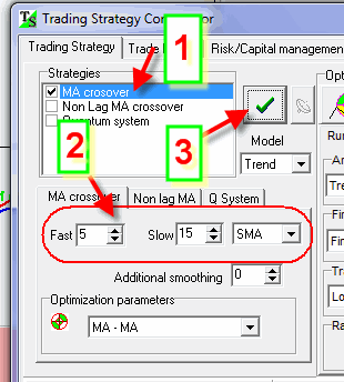
Immediately the program will display on the Main screen these moving averages (red - fast, blue - slow) and corresponding buy/sell signals:
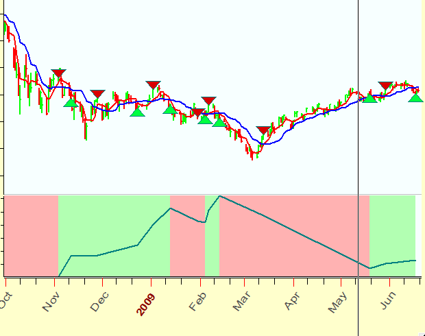
Also you will see the equity curve for this strategy (how profit may change in time) and all necessary information (profit, drawdown, win/loss ratio):

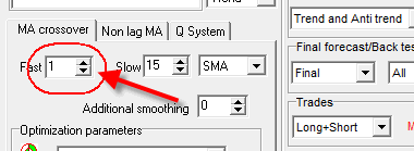
If you need to find the crossover of close and moving average, set the period for the fast moving average to 1:
Sure you can analyze all moving averages one by one finding the best one; this task can also be delegated to the program.
Simply click ![]() button; the program will analyze a lot of moving averages
finding for you the best ones. Moreover you can analyze all available trading strategies together clicking
this button
button; the program will analyze a lot of moving averages
finding for you the best ones. Moreover you can analyze all available trading strategies together clicking
this button ![]() :
:
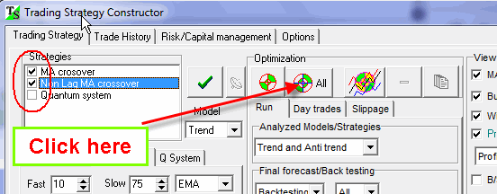
Then click on "Optimization" button (step 2 above), to make the program looking for the best available strategies.
In one minute the program analyzes 1.630 different trading strategies (in our example) based on different moving averages and finds the best ones (I have spent a lot of time developing fast algorithms for this step):
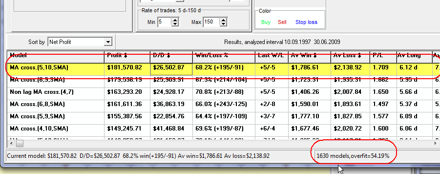
You can see that the best profit is provided by the strategy based on crossover of 5 and 10 days simple moving averages. This model (I used one $100K contract in this example) gives 181% profit (within 10 years), drawdown of this system is 26%. It provides 68% of winning trades; the average win is $1.786 while the average loss is $2.138
On the Main screen you can see the equity curve for this strategy and all buy/sell signals:
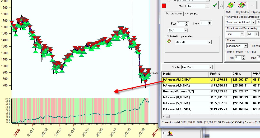
While the new price history is coming, the program recalculates buy/sell signals. You can even use this system in real time; the signals generated by it can serve as buy/sell alerts.
I recommend to highlight these strategies one by one and watch how the equity curve changes; the program redraws the equity curve and buy/sell signals when you highlight another strategy. Thus, fast and easy, you can browse a lot of strategies to figure out which one works better for you.
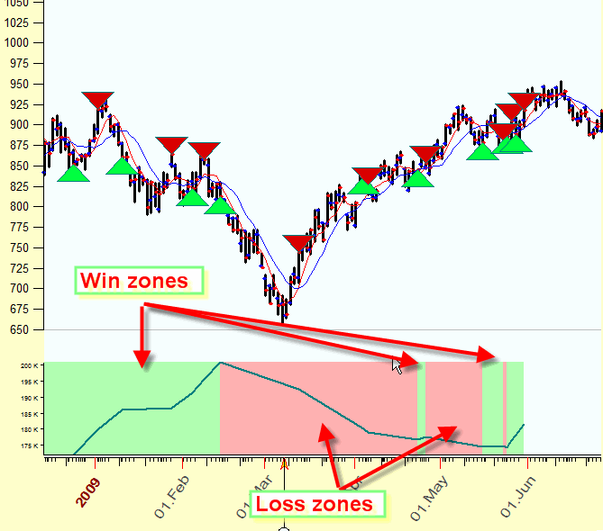
For your convenience, the win and loss zones are marked by green (win trades) and red (loss trades).
Also watch the "Last W/L" column. It shows the statistics of the last ten trades:
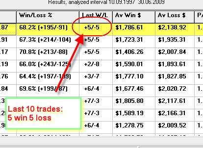
In our example above, the strategy provides 68.2% of winning trades (195 winning versus 91 losing trades). while the last ten trades give only half of this amount to winning trades (5 winning, 5 losing trades). Of course it may be some occasional fact.
Maybe it makes sense to deal with strategies that work well with the most recent price history and provide a steady growing equity curve. See this example; here the chosen strategy provides 7 winning trades versus 3 losing:
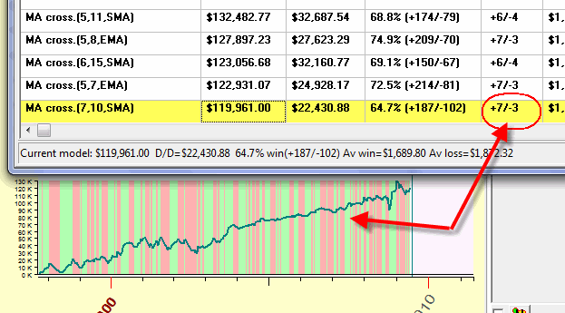
You can also sort these strategies by any criteria, like finding the strategies that provide the best win/loss ratio for the last 10 trades, or minimal drawdown or any other:
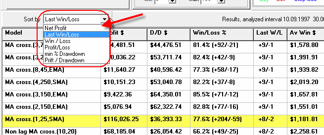
The whole trade history is available here:
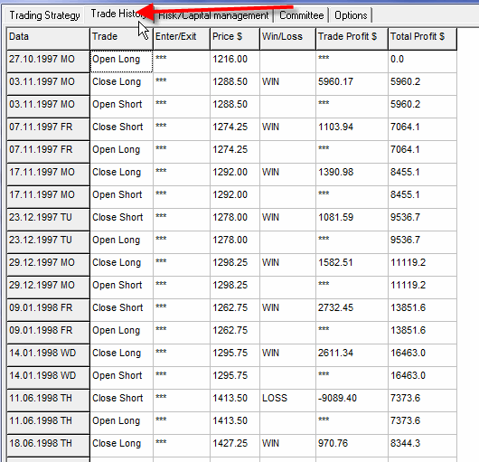
Important notice: while analyzing the equity curve, check it on different intervals with up and down trend. Watch how the equity curve comes through the periods of changing the trend,
How to pick up the best trading strategy
It took me a lot of time to think about formal criteria of choosing the trading strategy. Finally I figured out that for this particular case it is better to use non-formal criteria. Intuition can help here a lot. The reason is very simple: the human eye, in combination with the brain, skills and trading experience, can see the nuances that are practically impossible to catch using formal criteria. Timing Solution (and TSC module) provides very easy and convenient way of visualization all this information. Within just a few minutes you can browse hundreds of trading strategies and get a good impression of how these strategy work. There is nothing mystical here, simply the program performs some tasks that look very easy while being extremely complicated from a formal point of view.
The main rules are:
#1) Watch equity curves. A good equity curve should provide steady year-by-year (or day-by-day for intraday trading) growing profit;
#2) Check your model on different trends up and down, it is very important to know how your system overcomes periods with different trend. To do that look on the equity curve together with the corresponding price chart;
#3) Watch flat zones, i.e. the periods when your system does not provide any profit should not be big; especially pay attention to the latest price history;
#4) Be careful with parabolic/exponential equity curves when the profit grows very fast. These model stop working suddenly (when you deal with other software that provides exponential equity curves, this is a good sign that this system contains "future leaks". In Timing Solution future leaks are excluded).
It is preferable to deal with the strategy that provides steady growing equity curve, like this one:
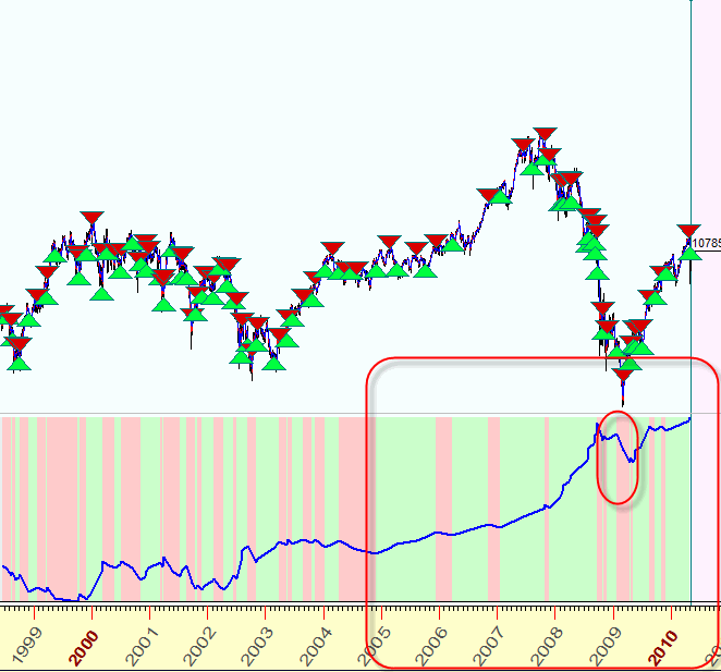
This model gives a a good profit curve for the last 5 years; drawdown in the end of 2008 - beginning of 2009 is the price for the financial turmoil.
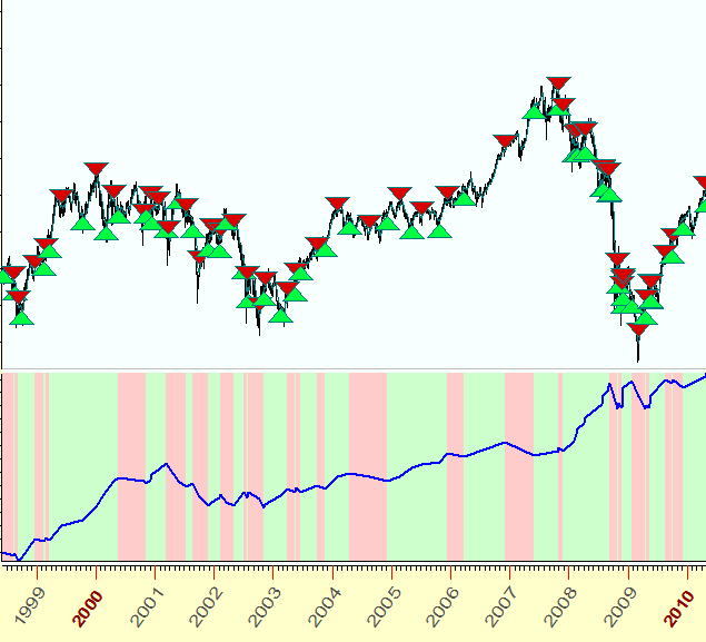
This is another good example:
Now look at one more equity curve:
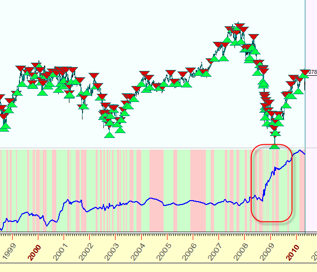
This equity curve provides a big profit while Great Financial Crisis is in force, extreme conditions lead to extreme profit (or loss). Personally I would be very cautious to use this model in the future. Usually such models stop working very sharp and suddenly.
Let's look at another equity curve:
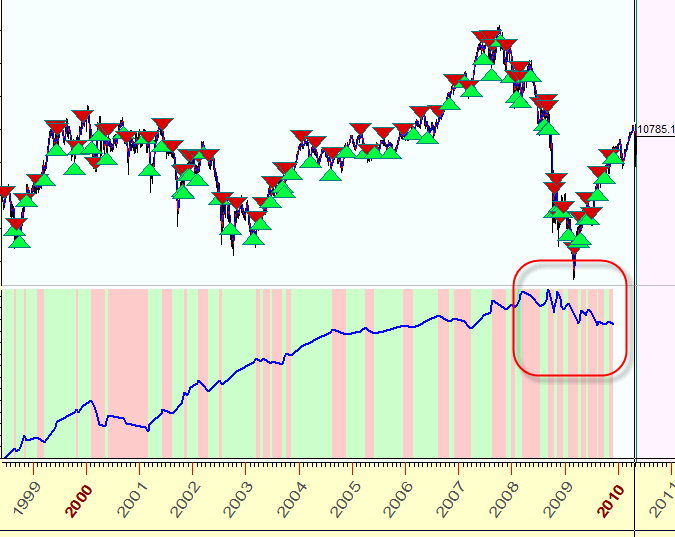
It provided a good profit till 2008; since the year 2008 the profit dropped. It looks like this model is loosing its profitability, it does not describe well the latest stock market behavior.
Committee strategy - dominant strategies
The idea of committee is very simple: we trade applying not just one moving average crossover, but using a bunch of moving averages or a bunch of other strategies trying to create the best trading strategy. Simply click this button:
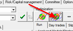
and in a moment the program redraws the buy/sell signals and equity curves for this committee strategy. The information regarding all involved strategies is displayed in the bottom of this window:

This committee strategy provides 124% profit; though the drawdown is huge (34%), it makes 83.9% winning trades.
This line: ![]() represents mathematical properties of the committee strategy. The program
performs very complicated calculations; for our example, it has found 35 best
moving average crossovers that provide best equity curves on 100 bars interval,
together with the best profit and win loss ratio. The program tries different
criteria (profit, win/loss ratio, profit factor) on different intervals and in
different combinations; it
compares these crossovers and finds the best parameters for committee strategy,
i.e. the strategy that provides the best profit.
represents mathematical properties of the committee strategy. The program
performs very complicated calculations; for our example, it has found 35 best
moving average crossovers that provide best equity curves on 100 bars interval,
together with the best profit and win loss ratio. The program tries different
criteria (profit, win/loss ratio, profit factor) on different intervals and in
different combinations; it
compares these crossovers and finds the best parameters for committee strategy,
i.e. the strategy that provides the best profit.
Technically the committee technology is very close to the technology of finding the dominant cycle for financial data; the only difference is that we are looking for dominant moving averages. However, I do not think that the main stream of Timing Solution technology is a committee method in spite the fact that the application of the committee strategy sometimes allows to decrease drawdown. I believe that developing new moving averages based on projection lines is more promising. Using strategies based on NON LAG moving averages is the first step in this direction.
I use the committee technology mostly for filtering. During the committee's calculation, the program performs the intensive back testing and finds the most efficient combination of strategies, like in the example above. There, among 659 analyzed models (the strategies with a positive profit), the program has found 35 most effective ones. You can delete all other strategies and leave only these the most important ones by clicking on this button:
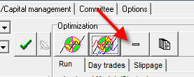
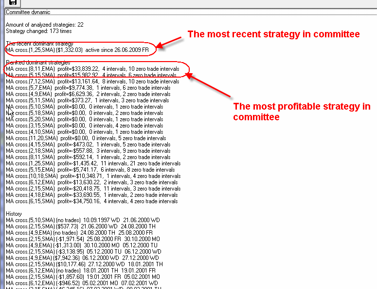
Clicking the next button, you can display the committee dynamics, i.e. to be able to see:
- the most recent strategy in the committee;
- the most profitable strategy in the committee;
- how dominant strategies changed in time:
Always pay attention to "Rate of trades" options:
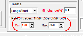
For example if you have downloaded 1 min price chart and look for the trading system that makes one trade in 2-6 hours, these options should be set up as on the picture above. It means that the average length of a trade will be in this range.
Also this option is important:
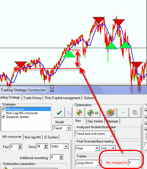
It shows the minimal price change between consequent trades. If this value is too small, you can face the effect of "phantom" trades, like here:
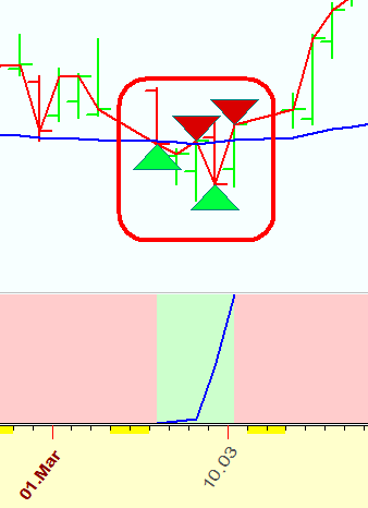
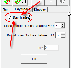
If you are a day trader, set this option ON:
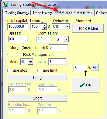
Risk management and commission. With this program, you can apply risk management techniques for your strategies such as stop loss orders and stop limits. Also do not forget to define the commission here, this is important. You can get a very impressive system with good enough gross profit, and this profit might disappear after applying the commission values (i.e. net profit might be zero). This is especially important for intraday trading. So please define risk management parameters and commission here:
Slippage. This is another important parameter, especially for intraday trading. The difference between the trade price and execution cost may be very significant especially for volatile markets:
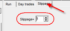
The slippage strongly depends on your broker. In Timing Solution the slippage is measured in bars, i.e. as an execution bar we use the next price bar if the slippage is equal 1.
In "Options' tab check this menu:
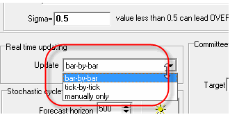

Below is the list of strategies that are available in this module now (April 2010).
- moving averages: this is a classical strategy based on the fast and slow (or close and moving average) crossover.
Here are the parameters for moving averages strategy:
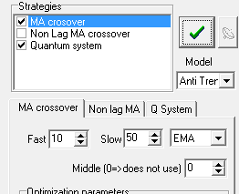
Define here the periods of fast and slow moving averages as well as a type of smoothing procedure (simple/exponential).
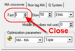
If you prefer using the simplest strategy of crossover of the price and the moving average, set the period for the fast moving average to 1:
You can also create the strategy based on triple moving averages. For example this is a classical triple moving average (Fast=4, Middle=9, Slow=18):
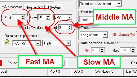
If the period of the middle moving average is set to zero, the program uses crossover of two moving averages.
You can optimize the triple moving averages highlighting this item:
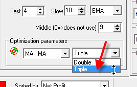
- non lag moving averages: this strategy is based on the crossover of two non lag moving averages (or close and moving average).
The most important issue in this system is to avoid future leaks, i.e. avoid using future price history while you create your trading system. We guarantee that the algorithms used in this module have no future leaks.
I am often asked whether future leaks are really important. My answer is: yes, they are. For example, look at the picture below. There you can see two regular non lag moving averages (they are created with future leaks): red - the fast one and blue - the slow one. However the crossover of these two (circled) does not indicate the buy signal:
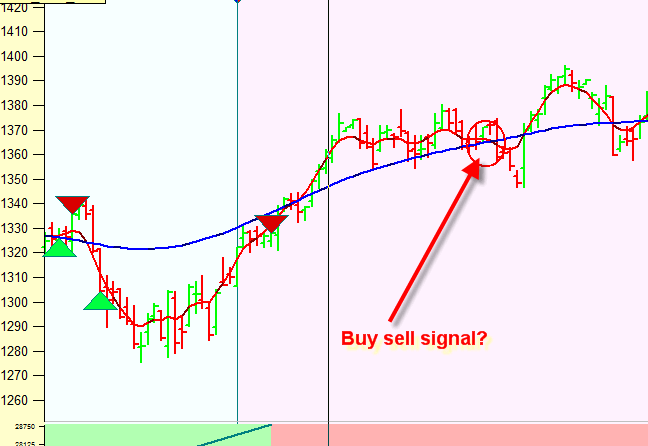
Why? Look at the same chart, now without future leaks. These are still the same fast and slow moving averages (thin red and blue lines), but the price aftere LBC is totally excluded from the calculation. In other words, this is how these non lag moving averages look at the moment (LBC moment) when we do not know the future price history (thick lines):
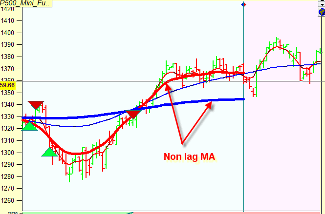
As you see the moving averages on the previous picture actually do not indicate a buy signal.
The parameters for non lag moving averages are the same as for the classical moving averages crossover.
- quantum strategy: this strategy presumes the existence of smallest quantities of the trend change. Quantum moving average shows the price movement in terms of quantum arithmetics:
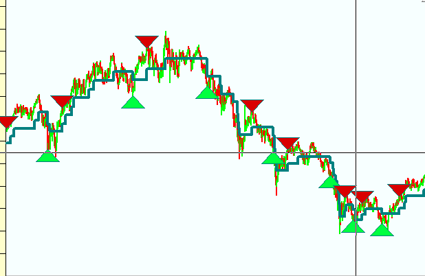
There are two parameters for the quantum model:
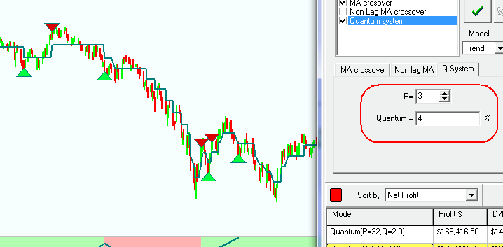
Quantum - is the value of the quantum; the bigger the value of quantum is, the bigger is the "step" in quantum moving average indicator.
P parameter makes the quantum moving average smoother.
This module is still under construction, and we do not describe all technical issues regarding the quantum system. The most important question here is to find the appropriate domain for the quantum analysis (price, time or both).
Technical Analysis Quantum Functions
In this section I will explain some details of creating quantum models, to make you able to create your own quantum models. As an example, consider True Range Breakout Model. True Range is a difference between High and Low, it shows how volatile the stock market is within a day.
From the point of view of quantum module, True Range Breakout models sound this way:
When the true range is higher than its average level, the trend TENDS to change, so this is a potential buy or sell point.
There is a very important statement inside this one; it is "TENDS to change". It means that the trend may change, and also it may not change at all. We simply say here that these moments are important, and we have to pay attention to these moments, they are potential decision points.
What does the quantum module do? In this particular example, it considers the moments when the true range is higher than the average value; the applied quantum model shows these moments as the moments when the quantum moving average jumps from one level to another, like here:
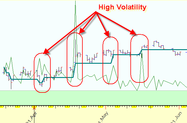
There is a very close analogy with physics, where the electron absorbs some energy and jumps to another energetic level. High volatility in our example indicates the moments when the quantum moving average jumps from one level to another.
If this jump confirms the existing trend (for example, up jump in the up trend market), we do not perform any action as the trend does not change. Otherwise if the jump is opposite to the existing trend, the program generates buy or sell signal, i.e. this quantum model sees the trend changing:
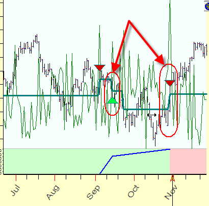
This is a beauty of the quantum system: we consider the moments when trend MAY change (the consideration is done by some quantum model), and the program provides the "quantum analysis" for this system (i.e. finds the value of quanta and noise filtering). As the result you get buy/sell signals ready for a trade and the equity curve that shows the past performance of this model.
Now it is the time to learn the technique.
First of all, you must define True range. Type this formula (follow the steps):
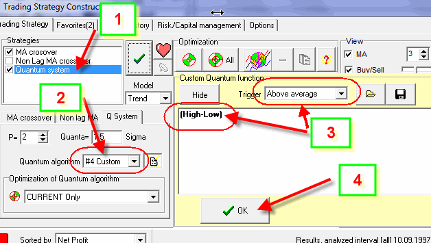
You can see the true range directly in the Main screen:
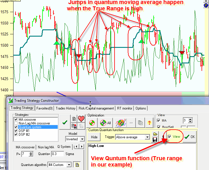
As you see the jumps of the quantum moving average happen when the volatility is high.
We call this function a quantum function; it points at the moments when the quantum moving average jumps from one price level to another. In other words this function triggers jumps in the quantum moving averages.
The last step is the optimization procedure: we order the program to find the best parameters for a quantum model that generates the maximum profitable strategy. Click this button, and you will get the list of rated strategies based on your True Range model:
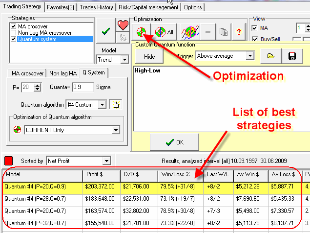
In the example above True Range breakout model was considered. There the high volatility triggers the quantum signal that can be taken as a buy/sell signal. There are also other criteria of triggering a quantum signal.
So far there are three criteria of triggering quantum signals in the program:
 variant. In other words, when True
Range exceeds some specific level, the quantum moving average jumps from one
level to another. You do not need to worry about what this level is: during the
optimization procedure the program finds this level automatically. The
measure of this level is a statistical parameter SIGMA, i.e. the deviation from
the average level.
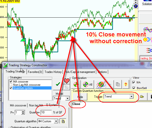
You can define the formula yourself. Below are examples how to build quantum formula:
Example A : Momentum based formula
Start with this one: the absolute value of the momentum exceeds 3 Sigma average level:
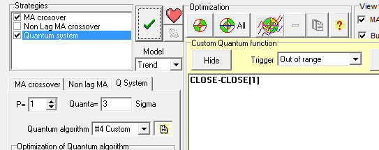
Momentum is a difference between the current and the previous price; the current price is CLOSE, while the previous price is CLOSE[1]. Thus the momentum can be defined as:
CLOSE-CLOSE[1]
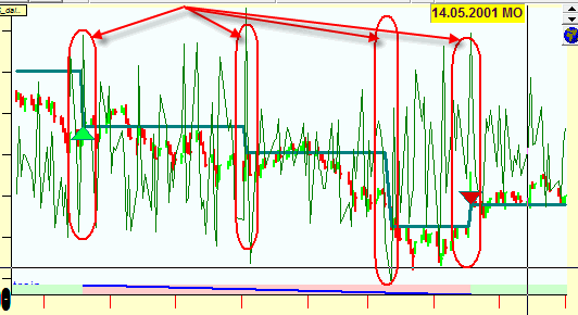
Thus the jumps of the quantum moving average take place when the absolute value of the momentum is high:
If you want to calculate a smoothed momentum, i.e. find the difference between the current price and the price several days ago, use this formula (as an example, let the previous price be the close 5 days ago):
CLOSE-CLOSE[5]
If you prefer to deal with normalized values, i.e. to calculate the price change in % (not in $), use this formula:
100*(CLOSE-CLOSE[1])/CLOSE
You can calculate the momentum for HIGH, like this:
HIGH-HIGH[3]
or use mixed momentum, like a difference between current HIGH and LOW 5 days ago:
HIGH-LOW[5]
You can also calculate VOLUME momentum:
VOLUME-VOLUME[1]
You can use more complicated formula as well. As an example, find the square of the momentum SQR:
SQR(CLOSE-CLOSE[1])
Or the absolute value (positive value) of the momentum ABS:
ABS(CLOSE-CLOSE[1])
Or the square root of the absolute value of the momentum SQRT:
SQRT(ABS(CLOSE-CLOSE[1]))
Example B: Energy based formula
You may like to see when the cumulative energy of Close is increased by 5%:
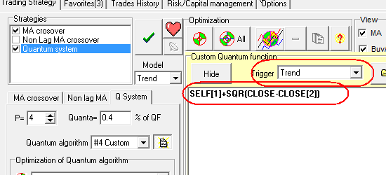
I use this definition here:
energy of the stock price is the square of the momentum, i.e. SQRT(CLOSE-CLOSE[1]). Again, it has the analogy in physics where the kinetic energy is a superposition of the mass and the square of speed divided by two. The speed is definitely the momentum, but what is the mass?
I tried to use VOLUME as a mass, so under this analogy the current kinetic energy of the stock market is: (m*v^2/2):
SQR(CLOSE-CLOSE[1])*VOLUME/2
However, I have found that this formula without volume works better (smoothed momentum CLOSE-CLOSE[2]):
SQR(CLOSE-CLOSE[2])
The full formula looks:
SELF[1]+SQR(CLOSE-CLOSE[2])
What is SELF[i]? In the calculation of the cumulative energy, we take the previous value of our quantum function (i.e. SELF[1]) and add it to the current kinetic energy of the stock market (i.e. SQR(CLOSE-CLOSE[2])). In other words this formula means: the cumulative energy today is the sum of yesterday's cumulative energy plus the energy of the stock market.
BTW, look at the equity curve provided by this model: for SNP 500 mini futures 100K contract, it gives 312K profit within 11 years, win loss ratio is 74,6%:
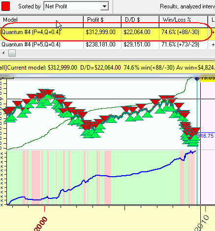
How do I check these formulas? This is what I do: type the formula, then press "Optimization" button to find the best quantum model based on this formula and watch equity curves for this strategy Then try some other formula..
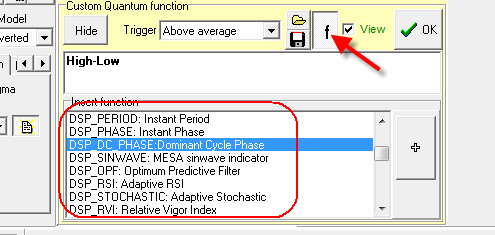
Now I will show the list of all functions that you can use to creatie customized quantum models.
BTW, you can see the list of all of them pushing "f" button:
Example C: Exponential moving average trend system
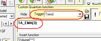
Set the quantum function as TA_EMA(3) and the trigger Trend:
The jumps to another price level in the quantum moving average appear when the change of value of the moving average reaches some specific value (quanta):
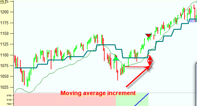
In other words the speed of the trade is defined by the speed of the changing moving average value.
I would recommend to vary the period of moving average, set it TA_EMA(3), TA_EMA(5), TA_EMA(10) etc.
You can use the simple moving average, like this TA_SMA(7), in the same manner.
Example D: RSI break out system
Set the quantum function as TA_EMA(14) and the trigger Out of range:

This model is based on the classical system that generates buy/sell signals when Relative Strength Index (RSI) breaks oversold/overbought levels. But here we combine this system with quantum models, the quantum moving average jumps to another price level when, when RSI breaks overbought/oversold levels.
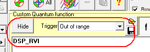
I would recommend to vary the period of RSI, set it TA_RSI(7), TA_EMA(14), TA_EMA(30) etc.
Example E: Bollinger band break out system
Set the quantum function as BOLLINGER_BAND(14) and the trigger Out of range:
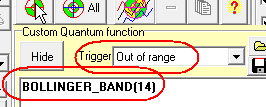
It works the same way as RSI break out system, the signals appear when the price breaks Bollinger bands. I recommend to vary the period for Bollinger band.
Remember that sigma (which is the range for Bollinger bands) is optimized by the program automatically.
Example F: Moving averages divergence break out system
Set quantum function as TA_EMA(7)-TA_EMA(20) and trigger Out of range:
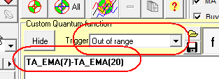
This system makes a trade when the difference between two exponential moving averages reaches some specific level. The quantum algorithms find the value of this critical level.
I would recommend to vary the periods of moving averages. Also try to play with divergence between Close and the moving average, like this one: Close-TA_EMA(5)
You can customize the quantum function using planetary positions. You can use these astro functions:
**************Geocentic position ***************
SUN:Sun position geo
MOON
MERCURY
VENUS
MARS
JUPITER
SATURN
URANUS
NEPTUNE
PLUTO
*************** Heliocentric position ****************
SUNH Earth position Helio
MERCURYH Mercury position Helio
VENUSH Venus position Helio
MARSH
JUPITERH
SATURNH
URANUSH
NEPTUNEH
PLUTOH
**************Declination***************
SUN_DEC :Sun declination
MOON_DEC :Moon declination
MERCURY_DECL Mercury declination
VENUS_DECL Venus declination
MARS_DECL
JUPITER_DECL
SATURN_DECL
URANUS_DECL
NEPTUNE_DECL
PLUTO_DECL
*************Geocentric for First price bar******************
SUN0:Sun position for FIRST price bar
MOON0:Moon position for FIRST price bar
MERCURY0:Mercury position for FIRST price bar
VENUS0:Venus position for FIRST price bar
MARS0:Mars position for FIRST price bar
JUPITER0:Jupiter position for FIRST price bar
SATURN0:Saturn position for FIRST price bar
URANUS0:Uranus position for FIRST price bar
NEPTUNE0:Neptune position for FIRST price bar
PLUTO0:Pluto position for FIRST price bar
*************Heliocentric for First price bar******************
SUNH0:Earth position Helio for FIRST price bar
MERCURYH0:Mercury position Helio for FIRST price bar
VENUSH0:Venus position Helio for FIRST price bar
MARSH0:Mars position Helio for FIRST price bar
JUPITERH0:Jupiter position Helio for FIRST price bar
SATURNH0:Saturn position Helio for FIRST price bar
URANUSH0:Uranus position Helio for FIRST price bar
NEPTUNEH0:Neptune position Helio for FIRST price bar
PLUTOH0:Pluto position Helio for FIRST price bar
You can also create the events like this: MERCURY[1]; it is Mercury position 1 day ago (for daily data); or Mercury[7] - Mercury position 7 days ago. Thus the formula Mercury-Mercury[1] represents the speed of Mercury.
Example G: the Sun step quantum model
In this module quanta is the time period for the Sun travelling some specific amount of degrees.
Look at this quantum moving average:
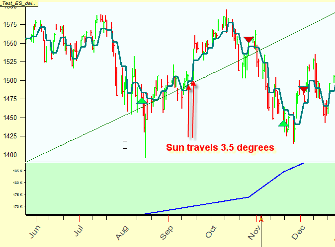
The quantum moving average jumps to another price level when the Sun travels 3.5 degrees of its arc starting from the previous jump. In other words we examine the potential turning points every 3.5 degrees of the Sun's movement.\
To calculate this model, type this quantum formula:
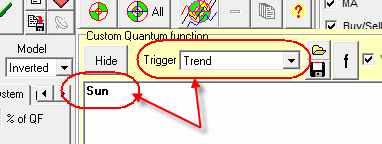
You should use "Trend" trigger here, because we deal here with the constantly increasing value which is the Sun position in the sky. After clicking "Optimize" button, the quantum algorithm finds the optimal step of the Sun movement. You can see this step in this information panel:

Example H: Mercury speed breakout models
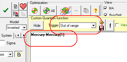
The idea of this model is that the quantum moving average jumps to another price level when the speed of Mercury is high (whatever Mercury movement is, direct or retrograde). The quantum algorithm finds the optimal values of critical Mercury speed. To create this model, define Mercury-Mercury[1] quantum formula and "Out of range" trigger criteria:
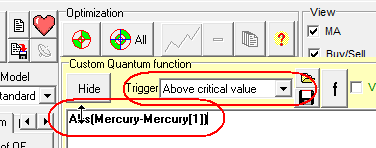
Another variation of this model is to use the absolute values of Mercury speed (Abs function) and "Above critical value":
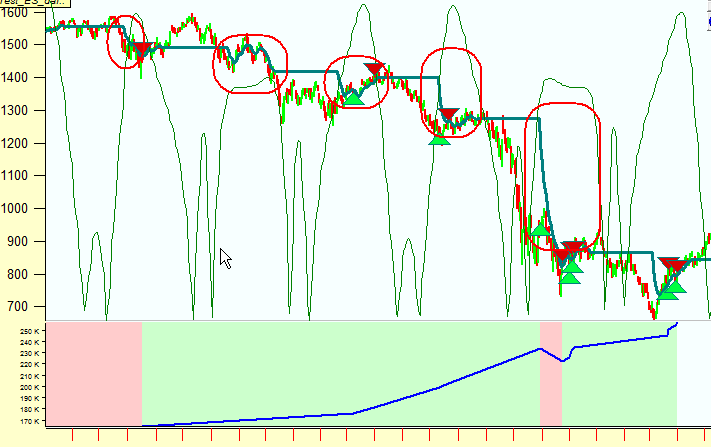
The quantum algorithm finds the optimal values for this critical value. The picture below shows the quantum moving average jumps when the speed (our custom quantum function) is high.
You can make the quantum function sharper or smoother using Power function, like this:
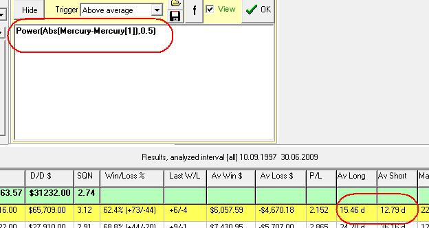
This way you can increase the amount of trades your model does.
Try to use these variations of quantum functions:
Power(Mercury-Mercury[1],0.1)
Power(Mercury-Mercury[1],0.2)
Power(Mercury-Mercury[1],0.5)
Power(Mercury-Mercury[1],0.75)
Power(Mercury-Mercury[1],1.5)
Power(Mercury-Mercury[1],2.0)
.....
Example I: Mercury-Venus speed breakout model
This model works exactly in the same manner as the previous model; the difference is that we use this quantum function:
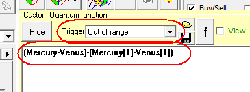
Try to use two variations of the formula: as above and Abs((Mercury-Venus)-(Mercury[1]-Venus[1])) quantum function together with "Above critical value" trigger criteria:

Example J: Mercury declination is high
You can create this model either this way:

or this:

Example K: the Moon phase model
You can create the Moon phase model this way (the Moon phase is the angle between the Moon and the Sun):
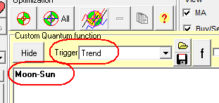
The rate of trades depends here on the Moon phases.
If you would like to create the model that trades mostly around the New and Full Moon, use this formula (the trigger here is "out of range"):
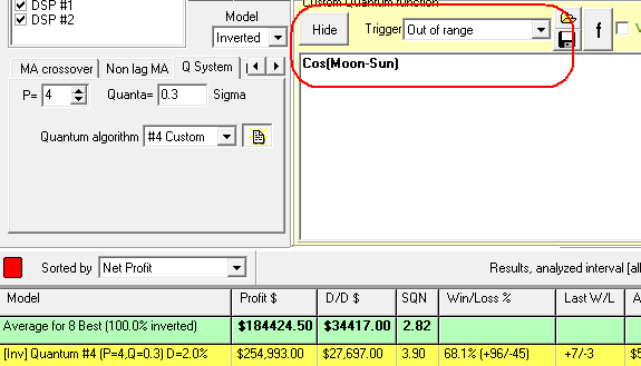
BTW, this model works not bad.
Vice versa if you are more interested in the model that does not trade around the New and Full Moons, set Sin(Moon-Sun) quantum function.
To calculate Mercury (and other planets) phase, use the difference between the heliocentric Mercury and the Earth, i.e. use this formula: MercuryH-SunH
Digital Signal Processing/MESA Quantum Function
You can create quantum trading system based on Digital Signal Processing (DSP) functions. You can read more about DSP here: http://www.timingsolution.com/TI/2/index.htm
All DSP functions are available through "f" button:
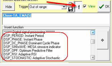
Example L: Dominant cycle period breakup model
Make more trades when the period of the dominant cycle is high (i.e. trade on long term cycles and avoid to trade on short term cycles because they are more noisy):
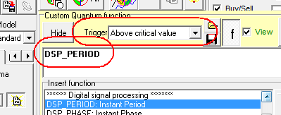
For this model, you should use Above critical value trigger criteria. The quantum algorithm finds this optimal level and shows it:

It means that the best trading strategy is provided when we trade on dominant cycles with the period higher than 28.5 bars.
If you prefer to trade on short term cycles, set "minus" quantum function -DSP_PERIOD
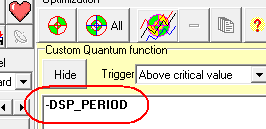
This is just an example of applying different formula for quantum functions; I did not find any good strategy with this particular approach, at least for daily data.
Example M: Cumulative dominant cycle period quantum model
The previous model did not provide a good strategy. I guess this is because these models are "breakup". For example, it trades when the dominant cycle period is higher than 28 bars, otherwise there is no trade.
Let's try more even model, it will trade MORE OFTEN on long term cycles. Let's say that it trades five times faster on the dominant cycle with the period 50 bars than on the dominant cycle with the period of 10 bars.
This is how this model looks:

You will see that this model trades on the whole interval. As a quantum function it uses the sum of the dominant period. To improve this model, try to use Power function, something like this:
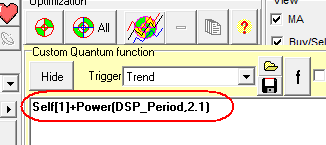
I recommend to vary Power function parameters, try:
Self[1]+Power(DSP_Period,1)
Self[1]+Power(DSP_Period,1.1)
Self[1]+Power(DSP_Period,1.2)
Self[1]+Power(DSP_Period,1.3)
Self[1]+Power(DSP_Period,1.4)
etc.
Power function makes the quantum function sharper.
To trade more often on short term cycles, try this quantum function:

Example N: Dominant cycle phase model
DSP dominant cycle model can be compared to the spinning wheel, and the speed of rotation of this wheel is constantly changing. This model adjusts the rate of trades with the phase of this "wheel":

For example, the quantum moving average jumps to another price level every time when this "wheel" covers 120 degrees of arc.
In this example we have considered an INSTANT phase. Using DSP_DC_PHASE you can create the model that employs Dominant Cycle phase (this is not the same as an instant phase). Dominant cycle phase shows how the price reacts on the rotation of this "wheel".
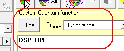
Example O: DSP breakout quantum models
These models work the same way as RSI breakout model, i.e. the model makes trade when RSI or other index breaks some overbuy/oversell levels.
We can create breakout system which is based on:
SinWave indicator

Optimum predictive filter
Adaptive RSI breakout system:

Relative Vigor index:
This is an extremely useful parameter to describe the quality of some trading strategy. It is surprisingly good in combining in one digit the profit and the risk. Now I use this parameter a lot, and it is present in TSC module.
The higher parameter value means the higher quality of the trading system. This is the table of correspondence for SQN:
| SQN Score | Quality of the System |
| 1.6-1.9 | Poor but tradable |
| 2.0-2.4 | Average |
| 2.5-2.9 | Good |
| 3.0-5.0 | Excellent |
| 5.0-6.9 | Superb |
| 7.0- | Holy Grail |
This parameter has been invented by Van K. Tharp, see his book "Super Trader".
I would like to mention that for intraday trading strategies the value of SQN is lower, because of a higher risk.
Stable solution
We have to start to think not in terms of a single good strategy, but in terms of a working technology. I will explain this problem using an example. In the previous section (Work in process, May, 2010) we have discussed how to create the cumulative energy model; here it is:
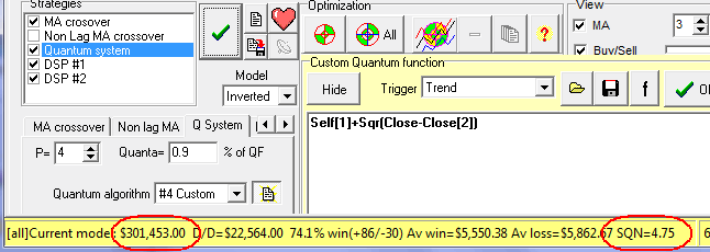
After the optimization, the program has found one very good strategy based on the cumulative energy: the profit is high, SQN (system quality factor) is excellent. Now try to vary one of the parameters of this model, let it be setting smoothing P factor to 3; you will see that the quality of this trading strategy drops significantly:

Why does it happen? The answer is simple - this model appears occasionally, we can take it as Game of Chaos. This is the result of over fitting effect, and now we try to figure out how to overcome this problem.
Transiting from best strategy to best technology
What was written above relates to our work in terms of best strategies. And the program is designed to find the best strategy. It meant that no matter how many strategies are considered, the program chooses the best one. As I have mentioned above, the biggest problem with this approach is over fitting. To avoid this problem, we need to change the technology of looking for best strategies.
The new approach is: after downloading some financial instrument data (E-mini futures daily in our example), we watch how the strategies based on moving averages crossover work (we do not consider here the strategies of other types - only moving averages). Click this button:
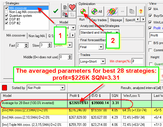
The program shows the average profit/draw down/system quality number for 28 best strategies based on moving averages.
In other words the program picks up 28 best strategies from 556 considered and calculates the average profit, drawdown, system quality factor for them. This parameter is more stable than a single strategy. Among these best strategies we have a very good strategy with SQN=4.29 and the profit=$267K; however, we keep ourselves calm in regards to this strategy: this super strategy might turn to be just another Game of Chaos. We are looking parameters we can trust.
Now, try to vary this parameter:
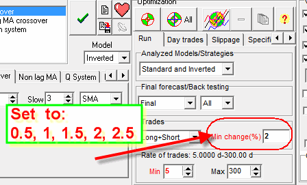
Set the minimal price change between the trades to 0.5, 1.0, 1.5, 2.5, 3; click "Optimize" button and watch how the quality of these strategies is changing. I decided not to perform this procedure automatically because it is better to watch these strategies manually. For example, if you set min change parameter to 2.4%, you get a higher profit and higher SQN:

However, as you see, this strategy is too "lazy": in total it makes not too many trades (the win/loss ratio of +78/-29 means that 78+29=107 trades have been done). And it means that a random error is higher, so I would prefer to deal with the system that generates more trades (like the previous strategy with "default" min change=2%).
Put this figure in the table.
When we completed the research for strategies based on moving averages, we may conduct the same analysis for non lag moving averages strategies and add these digits to the table:
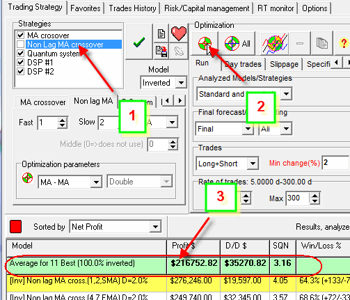
The result is not so good.
Then we may try strategies based on Quantum trend model:
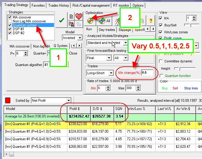
There you see the best SQN=3.54 for min change parameter = 0.5. Now this is the best model.
Pay attention: now the program analyzes 26 best models (not 28 as it was for moving averages strategies). This is because it takes 15% from ALL analyzed profitable strategies. This way we put all analyzed strategies into equal position. Otherwise we will have dominating strategies that are based on moving averages (just because this method provides the biggest amount of strategies).
Now I recommend to check the set of Custom Quantum models. Click this button and check these models one by one (do not forget to vary min change parameter):
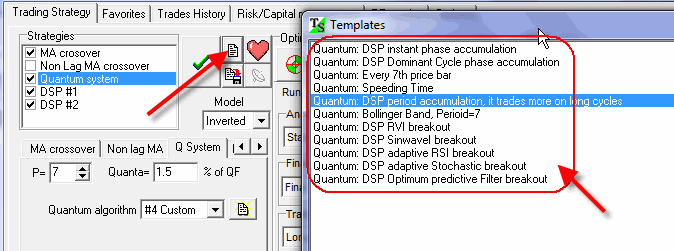
I have chosen the models that provide SQN 3 and higher.
Here they are:
 SQN=3.06 Min change=2%
Bollinger Band with smoothing period=10, type this custom formula  , min change=1% this model provide SQN=3.32
 SQN=3.43 min change=1.5%
This is the final table of the best strategies:
|
S&P500 mini future DAILY |
|||
| Model | Min Change(%) | Profit (x $1000) | SQN |
| MA crossover | 2 | 226 | 3.31 |
| Quantum (Trend) | 0.5 | 234 | 3.54 |
| Quantum (DSP: DC period accumulation) | 2 | 208 | 3.06 |
| Bollinger Band (10) | 1 | 234 | 3.32 |
| Quantum (DSP: Sinwave breakout) | 1.5 | 234 | 3.43 |
PLEASE REMEMBER THAT TIMING SOLUTION TERRA INCOGNITA PROJECT CREATES BUY/SELL SIGNALS IN ACCORDANCE WITH SOME THEORY. TO APPLY THESE SIGNALS TO YOUR TRADING IS YOUR DECISION. YOU, AND ONLY YOU, ARE RESPONSIBLE FOR IT. TIMING SOLUTION SOFTWARE, TS TERRA INCOGNITA PROJECT AS WELL AS THEIR DESIGNER AND OWNER HAVE NO RESPONSIBILITY FOR ANY DAMAGE THAT MAY OCCUR AS THE RESULT OF THAT DECISION OF YOURS.